> ## Documentation Index
> Fetch the complete documentation index at: https://docs.trlyr.com/llms.txt
> Use this file to discover all available pages before exploring further.
# Ramp Rates
An in-depth guide to how terralayr handles ramp rates in virtual assets.
This page covers what ramp rates are, terralayr’s design philosophy, the key variables, the cone of flexibility, governing equations, and practical examples.
# Introduction to Ramp Rates
Before diving into the details, let's clarify what a **ramp rate** is.
Unlike conventional power plants, BESS can adjust their power output extremely fast and flexibly. This would create high stresses on the grid, so in order to mitigate those and ensure stable operations, both DSOs and TSOs impose ramp rate restrictions on batteries.
In simple terms, a ramp rate is the speed at which a battery is allowed to increase and decrease its power output. Just as a car cannot instantly accelerate from 0 to 100 miles per hour, effectively a battery cannot instantly switch from full charging to full discharging.
Our virtual assets are always physically backed, meaning they inherit some of the real world’s physical limitations. Consequently, every virtual asset has its own ramp rate. Our job at terralayr is to translate these complex physical limitations into predictable and digestible rules for you. This document outlines how we have done that, providing a framework that enables you to confidently interact with the virtual asset without delving into the technical details of the hardware.
Our system operates on a "cone of flexibility" principle. This cone represents the range of possible power schedules you can submit for a future time period. As a quarter-hour delivery period approaches, the cone narrows, meaning the range of possible schedules decreases.
# Design Philosophy and Underlying Assumptions
This section explains how we arrived at our implementation of virtual ramp rates by detailing our design philosophy and the underlying assumptions.
## Design Philosophy
Our implementation of ramp rates is based on the following guiding principles:
* Ensure all market regulations are strictly adhered to, incl. e.g.:
* the ramp-rate restriction itself
* the Ancillary Services 5-minute anticipated setpoint.
* Ensure the range of flexibility is clearly defined and predictable e.g.::
* you submit a schedule for a particular quarter-hour period to a 30 MW discharge.
* you change that schedule to 40 MW discharge.
* you then change that schedule back to a 30 MW discharge.
* the range of flexibility available to you now should be the same as before the changes.
* Ensure the range of flexibility is as wide as possible for as long as possible.
* Ensure that, should the desired dispatch lie outside of that range, such schedules are fulfilled as best as possible, ensuring that in such an event all risk borne by customers is transparent and clearly defined.
## **Underlying Assumptions:**
Each of these design philosophy choices leads to some underlying assumptions about the way the "cone” of available flexibility is calculated.
* **All Market Regulations Are Strictly Adhered To** Virtual Assets are always backed by physical reality. This means that the regulations that govern the operations of physical assets must also be applied to virtual assets. Ramp rates themselves are an example of this regulatory landscape, but another key example is the Ancillary Services 5-minute setpoint rule.
* For assets participating in Ancillary Services, the TSO requires that anticipated setpoints for power production/consumption are sent 5 minutes in advance.
* After this 5 minute deadline, dispatch schedules cannot be changed.
* For this reason, terralayr imposes a minimum gate closure of 5min30s for all final dispatch schedule submissions.
* This ensures that market rules are always adhered to.
* **The Range Of Flexibility Is Clearly Defined And Predictable** **Physical Reality:** In traditional ramp rate handling, asset behaviour is intransparent, depending on all previous dispatch schedule updates. Imagine the time is 12:16 and you are planning your dispatch schedule for the 12:30-12:45 settlement period:
* Your final trades for the 12:15-12:30 period have cleared, and any delivery profile for the 12:15-12:30 period must respect your cleared positions or you incur imbalance.
* In principle, if a schedule update is sent for the 12:30-12:45 settlement period the delivery profile could be recalculated from 12:21-12:30 to make the schedule update for 12:30-12:45 feasible.
* However, if you send another update to the schedule at 12:18, the delivery profile from 12:21-12:23 cannot be changed without breaking the ancillary services 5-minute anticipated setpoint rule, only the schedule from 12:23-12:30 can be changed.
* The final range of flexibility available for 12:30-12:45 therefore doesn’t just depend on the latest schedule value, but on the entire history of schedule updates.
* This leads to *hysteresis* in the range of available flexibility - the available range at gate closure is defined by the whole history of changes made to the schedule, and every time you update the schedule your range of available flexibility reduces.
* If virtual batteries supported continuous recalculation, they would inherit hysteresis from the underlying physical assets. This would mean that
* It is impossible to define a clear set of equations that wholly capture a virtual asset’s range of flexibility, which introduces unpredictability for customers.
* It is technically complex for both customers and terralayr to implement proper auditable logging of risk exposure and virtual asset capabilities.
* As a result, we do not currently believe that the benefits of continuous recalculation outweigh the significantly increased complexity and decreased transparency that it would lead to. **Virtual Assets:** Instead of optimising for continuous recalculation, we set defined times for dispatch profile (re-)calculation. At these (re-)calculation points, your currently submitted schedule is used as a *draft* schedule for the upcoming settlement period. On a best efforts basis, we will always try to centre your available flexibility on the draft schedule. This maximises the range of changes you can make to your schedule from one (re-)calculation point to the next, while keeping the range of flexibility predictable, transparent and non-hysteretic. Currently, our (re-)calculation points are:
* **Initial Calculation Point:** 16min30s before delivery start
* **Final Calculation Point:** 5min30s before delivery start (gate closure) For example, imagine the time is 12:16 and you are planning your dispatch schedule for the 12:30-12:45 settlement period.
* Your final trades for the 12:15-12:30 period have cleared, and any delivery profile for the 12:15-12:30 period must respect your cleared positions or you incur imbalance.
* Your draft schedule for 12:30-12:45 at 12:13:30 was used to centre your range of flexibility on 30 MW.
* You update the schedule from 30 MW to 40 MW.
* Since we are between the initial and final calculation points, this schedule update has no impact on your range of available flexibility you can access between 12:30-12:45. i.e. unlike a physical battery with continuous recalculation, you are able to change your schedule as much and as often as you like without impacting your range of available flexibility.
* Your final dispatch schedule at gate closure is then delivered in full from 12:30-12:45. By avoiding the operational complexities of continuous recalculation, we ensure that the range of available flexibility is at all times transparent and predictable, making risk exposure easier to track.
* **The Range Of Flexibility Is As Wide As Possible For As Long As Possible** **Physical Reality:** The above example that leads to an unpredictable and intransparent range of available flexibility also impacts the size of the range of flexibility you have access to. With continuous recalculation, not only is your range of flexibility hysteretic - depends on the entire history of schedule updates submitted - but every time a schedule update is sent, your range of flexibility is reduced. **Virtual Assets:** By only performing (re-)calculation at specific, pre-defined points in time, the range of available flexibility between those points remains unimpacted by schedule changes and stays as open as possible, for as long as possible.
* **All Customer Schedules Are Maximally Fulfilled And All Risks Borne By Customers Are Transparent And Clearly Defined** By utilising draft schedules at specific (re-)calculation points, we will always attempt to centre the range of available flexibility at the latest draft schedule. This maximises the range of changes you can make to your schedule up until gate closure which are physically deliverable. However, not all schedules will necessarily be physically deliverable without consequences. The two main delivery risks for customers are:
* **Imbalance risk:** a schedule for one settlement period is physically feasible, but not without incurring imbalance for another settlement period.
* **Overcycling Risk**: a schedule for one settlement period is physically feasible, but not without relying on counter-activation, which leads to overcycling of the asset. **Example**
* Imagine you have a 50 MW virtual asset and have scheduled a 50 MW dispatch for 12:15-12:30, and you want to schedule 0 MW for 12:30-12:45. What should the power of the asset at 12:30 be?
* Option 1
* The power of the asset at 12:30 is 50 MW.
* From 12:30-12:32:30 the asset ramps down from 50 MW → 0 MW.
* From 12:32:30 → 12:45 the asset needs to dispatch some negative power to counteract the power dispatched during the initial ramp down phase.
* No imbalance is incurred, but the total dispatched energy of the asset increases by approx. 1 MWh between 12:30 → 12:45 and the overall SoE of the asset decreases due to dispatch inefficiencies.
* Option 2
* From 12:27:30 → 12:30 the asset ramps down from 50 MW → 0 MW.
* From 12:30 → 12:45 the asset’s power output is 0 MW.
* No additional cycling is required to deliver the schedule, but there is imbalance incurred in the 12:15-12:30 settlement period These are fundamental risks that are the result of unalterable dispatch limitations of physical assets. We have a strict internal policy in place to ensure that any physical dispatch risks should be clearly defined, predictable and transparent before they are exposed to customers. This ensures customers can properly manage their risks internally. Disaggregating this risk from an entire portfolio physical assets across a wide range of customers in a fair, transparent, pre-determined way is a complex legal, contractual, and technical problem which we are actively working on.
# Interacting with Ramp-Limited Virtual Assets
This section summarises how ramp rates impact the way you can interact with a virtual asset's dispatch schedule in the base case, from submission to validation and implementation. It also describes how, when counter activation is needed, we calculate the associated cycling costs.
**What is Counter Activation?** Counter activation occurs when a dispatch profile requires an asset to transition from positive to negative power (or vice versa) within a single settlement period. This happens when the asset must cross the zero-power line, requiring both charging and discharging operations in the same 15-minute window to fulfil dispatch requirements.
1. **You Submit Schedules:** You send dispatch schedules to LAYR, specifying 15-minute average power for each settlement period in a trading day. You can submit any schedule within the asset's power limits. *We won't enforce ramp rate constraints until 7 minutes before delivery*.
2. **We Communicate Limits:** The range of possible power outputs for any period is determined entirely by the preceding quarter-hour and the virtual asset's ramp rate. We provide the exact limits in the "Governing Equations" section below.
3. **Schedules are Validated before Gate Closure:** You can submit and adjust schedules until Dispatch Schedule Gate Closure, after which your schedule is locked. If schedules exceed the allowed range, we'll adjust them 7 minutes before delivery to ensure they're physically deliverable, as outlined [here](/layrUserGuide/features/unavailabilities). Between the 7-minute validation and Gate Closure, only schedules that comply with ramp-rate restrictions will be accepted.
4. **Counter Activation Cycles Are Finalised**: Once the final schedule for the upcoming quarter hour and the boundary powers for both the preceding and upcoming quarter hour are fixed, we can calculate the additional charge/discharge energy from counter activation. This is applied to the virtual asset during the upcoming quarter hour.
# Key Variables
For each quarter-hour period ($Q_n$) we define 7 key variables that determine the range of available flexibility of a virtual asset. These variables have foundations in the underlying physical reality of BESS and can be understood by considering a physical asset’s quarter-hourly dispatch schedule.
 1. **Maximum Power** ($P_{max}^{ch/dsch}$): The **available** charge/discharge power capacity of the virtual asset, in MW.
2. **Rated Power** ($P_{rated}$): The maximum rated power capacity of the asset, in MW.
3. **Ramp Rate (**$r$**):** the ramp rate of the virtual asset in $\% P_{rated}$ per second.
4. **Final Schedule (**$P_{f,Qn}$**):** The final delivered power for quarter-hour $n$**,** in MW. This is fixed at gate closure, typically 5min30s before delivery.
5. **Initial Calculation Point (**$T_{d,Qn}$**):** The point in time that terralayr reads your draft schedule for quarter-hour $n$, typically 16min30s before delivery.
6. **Final Calculation Point (**$T_{f,Qn}$**):** Gate closure for quarter-hour $n$, typically 5min30s before delivery.
7. **Settlement Period Duration (**$T_{SP}$**):** The duration of a settlement period, in seconds. Currently 900s (15 minutes).
8. **Draft Schedule (**$P_{d,Qn}$**):** The schedule for quarter-hour $n$ submitted to terralayr by the **Initial Calculation Point,** in MW.
9. **Boundary Power (**$P_{b,Qn}$**):** The instantaneous power level at the end of quarter-hour $n$, in MW. On a best efforts basis, we will make the boundary power for a given quarter hour equal to the draft schedule for the following quarter hour. This ensures that the range of available flexibility at gate closure is always centred on your draft schedule.
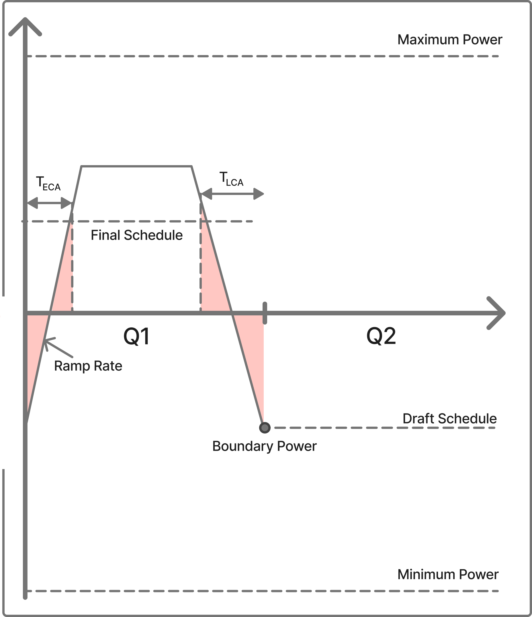
10. **Early Counter Activation Window** ($T_{ECA,Q_n}$): The window of time at the *start* of a settlement period where an asset is counter activating.
11. **Late Counter Activation Window** ($T_{LCA,Q_n}$): The window of time at the *end* of a settlement period where an asset is counter activating.
The Early and Late Counter Activation Windows are functions of the **boundary powers**, **rated power** and **ramp rate**:
```math theme={null}
T_{ECA,Q_n}\equiv\frac{200|P_{b,Q_{n-1}}|}{rP_{rated}}, \quad T_{LCA,Q_n}\equiv\frac{200|P_{b,Q_{n}}|}{rP_{rated}}
```
# Cone Of Flexibility - High Level Summary
terralayr describes the possible options for dispatch power into the future as a “cone of flexibility”. The further away a dispatch period is, the wider the cone of flexibility.
Your flexibility begins to decrease in the settlement period before delivery. The graph below shows how the cone of flexibility narrows as you approach gate closure for Q2 as a function of the draft schedule for Q2 submitted by the initial calculation point. We always try to keep the range of flexibility as big as possible.
For this high level summary section, and for the examples highlighted below, we assume the following:
* The maximum charge/discharge power of the virtual asset is equal to the rated power (i.e. no unavailabilities)
* The duration of a settlement period is 900s (15 minutes).
* The ramp rate is $0.66\% P_{rated}s^{-1}$**.**
For more detailed and fully generalised formulae that do not make these assumptions, see the [Governing Equations](/layrUserGuide/deep-dives/test#governing-equations) section below.
## Between Initial Calculation Point and Gate Closure for Q2
1. **Maximum Power** ($P_{max}^{ch/dsch}$): The **available** charge/discharge power capacity of the virtual asset, in MW.
2. **Rated Power** ($P_{rated}$): The maximum rated power capacity of the asset, in MW.
3. **Ramp Rate (**$r$**):** the ramp rate of the virtual asset in $\% P_{rated}$ per second.
4. **Final Schedule (**$P_{f,Qn}$**):** The final delivered power for quarter-hour $n$**,** in MW. This is fixed at gate closure, typically 5min30s before delivery.
5. **Initial Calculation Point (**$T_{d,Qn}$**):** The point in time that terralayr reads your draft schedule for quarter-hour $n$, typically 16min30s before delivery.
6. **Final Calculation Point (**$T_{f,Qn}$**):** Gate closure for quarter-hour $n$, typically 5min30s before delivery.
7. **Settlement Period Duration (**$T_{SP}$**):** The duration of a settlement period, in seconds. Currently 900s (15 minutes).
8. **Draft Schedule (**$P_{d,Qn}$**):** The schedule for quarter-hour $n$ submitted to terralayr by the **Initial Calculation Point,** in MW.
9. **Boundary Power (**$P_{b,Qn}$**):** The instantaneous power level at the end of quarter-hour $n$, in MW. On a best efforts basis, we will make the boundary power for a given quarter hour equal to the draft schedule for the following quarter hour. This ensures that the range of available flexibility at gate closure is always centred on your draft schedule.
10. **Early Counter Activation Window** ($T_{ECA,Q_n}$): The window of time at the *start* of a settlement period where an asset is counter activating.
11. **Late Counter Activation Window** ($T_{LCA,Q_n}$): The window of time at the *end* of a settlement period where an asset is counter activating.
The Early and Late Counter Activation Windows are functions of the **boundary powers**, **rated power** and **ramp rate**:
```math theme={null}
T_{ECA,Q_n}\equiv\frac{200|P_{b,Q_{n-1}}|}{rP_{rated}}, \quad T_{LCA,Q_n}\equiv\frac{200|P_{b,Q_{n}}|}{rP_{rated}}
```
# Cone Of Flexibility - High Level Summary
terralayr describes the possible options for dispatch power into the future as a “cone of flexibility”. The further away a dispatch period is, the wider the cone of flexibility.
Your flexibility begins to decrease in the settlement period before delivery. The graph below shows how the cone of flexibility narrows as you approach gate closure for Q2 as a function of the draft schedule for Q2 submitted by the initial calculation point. We always try to keep the range of flexibility as big as possible.
For this high level summary section, and for the examples highlighted below, we assume the following:
* The maximum charge/discharge power of the virtual asset is equal to the rated power (i.e. no unavailabilities)
* The duration of a settlement period is 900s (15 minutes).
* The ramp rate is $0.66\% P_{rated}s^{-1}$**.**
For more detailed and fully generalised formulae that do not make these assumptions, see the [Governing Equations](/layrUserGuide/deep-dives/test#governing-equations) section below.
## Between Initial Calculation Point and Gate Closure for Q2
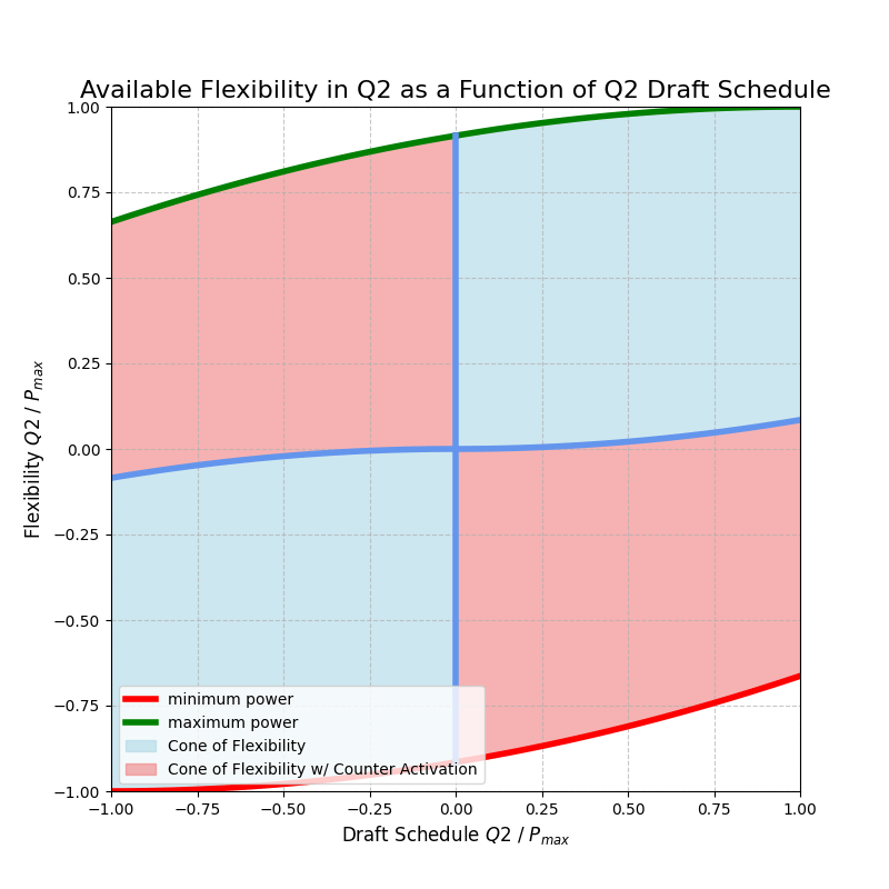 The total range of flexibility for Q2 is defined by the draft schedule for Q2 (submitted 16min30s before the start of Q2).
* If the draft schedule for Q2 is positive, the boundary power for Q1 will be positive. This means that to deliver a negative power, some level of counter activation is required.
* The opposite is also true (e.g. draft schedule for Q2 is negative)
* If the draft schedule for Q2 is 0, the boundary power for Q1 will be 0 and the range of available flexibility for Q2 is $\pm91.5 \% \times P_{max}$.
***
# Examples of Flexibility for a 50 MW Virtual Asset
Let's explore three practical examples to understand how flexibility works with a 50 MW virtual asset:
### Example 1: Using Full Rated Power
If you want to use the full rated power of your 50 MW virtual asset, you need to:
* Submit a draft schedule of 50 MW by the initial calculation point to ensure the system can prepare for maximum power output without incurring any imbalance.
* To avoid counter activation, ensure that the settlement period before the 50 MW dispatch has at least 4.2 MW of power scheduled to account for the energy discharged during the ramp up to 50 MW.
* This 4.2 MW minimum is a physically derived requirement, as the assets need to ramp up to 50 MW in the preceding settlement period.
* If the preceding settlement period has a scheduled power of less than 4.2 MW, counter activation will be required to ensure the asset can ramp up to the full 50 MW discharge power.
* Even after submitting a 50 MW draft schedule, you can still reduce this to as low as -33.2 MW between the initial calculation point and gate closure.
### Example 2: Undecided Between Charging and Discharging
If you're uncertain whether you want to charge or discharge at the initial calculation point:
* Submitting a 0 MW draft schedule still maintains maximum flexibility for minimal counter activations.
* This keeps open 45.75 MW (91.5% of 50 MW) in both charge and discharge directions, and incurs no additional charge/discharge energy due to counter activation.
* Submitting a positive draft schedule and a negative final schedule will incur additional discharge.
* Submitting a negative draft schedule and a positive final schedule will incur additional charge.
* A 0 MW draft schedule provides the optimal balance of flexibility, allowing you to decide the sign of your position up until gate closure.
### Example 3: Scheduling Something Not Deliverable
Consider this scenario:
* You've scheduled 50 MW for one settlement period, and this is being delivered
* For the next settlement period, you schedule -50 MW (charging)
* This schedule cannot be physically delivered - there is no way to swap from 100% charge to discharge within 2 settlement periods.
* We still accept the schedule initially, but at 7 minutes before delivery, we perform schedule validation
* During validation, we impose ramp rate constraints and adjust your schedule to the smallest deliverable value (-33.2 MW)
* This means your asset will be charging at -33.2 MW instead of charging at -50 MW as originally requested.
# Governing Equations
This section covers the detailed mathematical formulas that are used to define a customer’s range of available flexibility, and also how we calculate the additional charge/discharge energy values associated with counter activation.
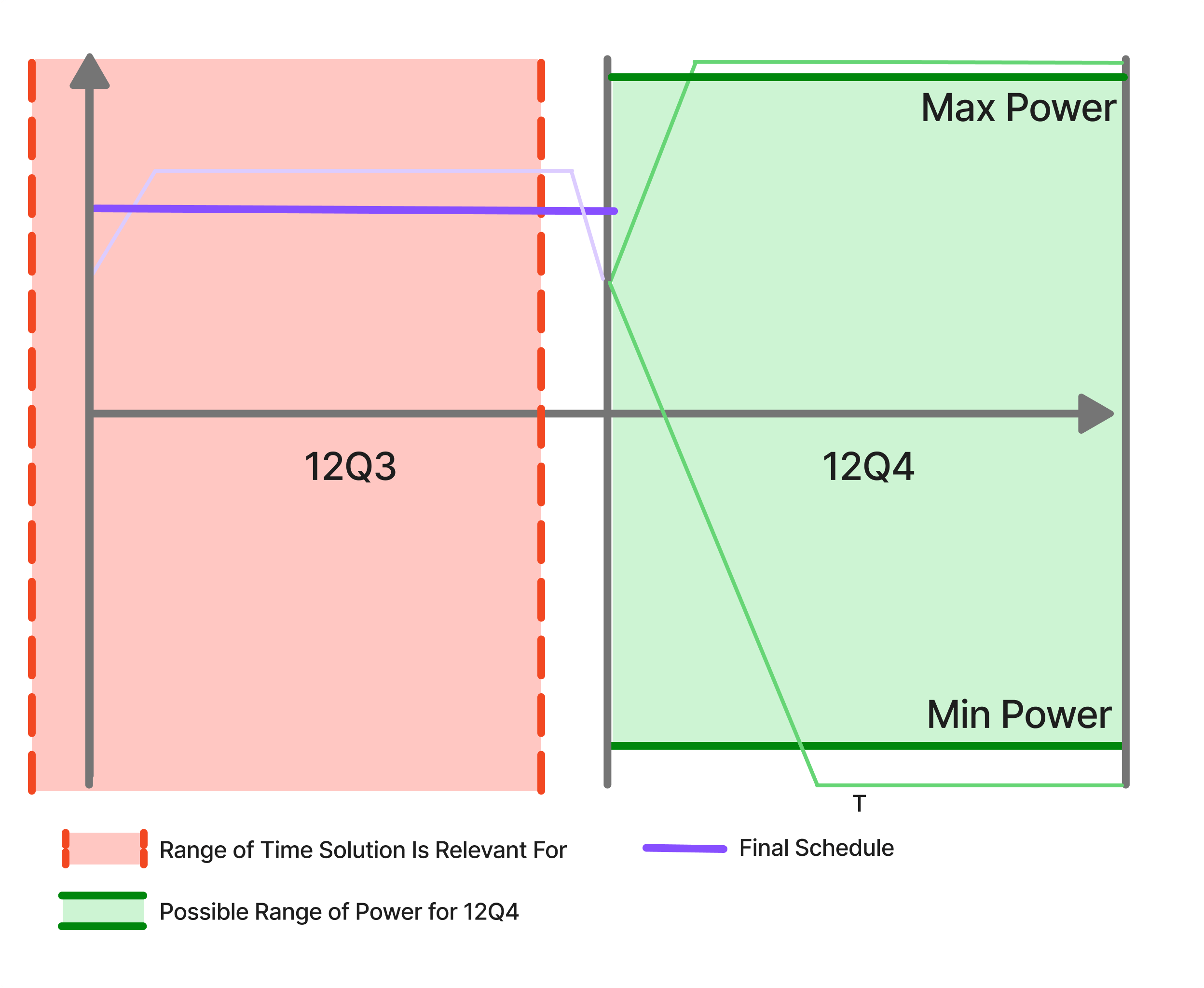
## Detailed User Journey
Imagine you are planning a schedule for 12Q4 (12:45 - 13:00).
The maximum and minimum power you can schedule for Q4 depends on the time relative to delivery.
### **Before Initial Calculation Point for Q4 (before 12:28:30):**
The range of flexibility for 12Q4 is fully open, allowing for any schedule within your virtual asset’s available power limits.
```math theme={null}
P_{Q4,max}=+P_{max},\quad P_{Q4,min}=−P_{max}
```
### **Between Initial Calculation Point for Q4 and Gate Closure (12:28:30-12:40:30):**
Your flexibility for Q4 is wholly defined by the draft schedule for Q4, the fixed **Boundary Power** of Q3 **(**$P_{b,Q3}$**)**
```math theme={null}
P_{Q4,max}=P_{b,Q3}+\frac{rP_{rated}T_{SP}}{200}-\frac{100}{2rP_{rated}T_{SP}}\left[\max\left(P_{b,Q3}+\frac{rP_{rated}T_{SP}}{100}-P_{max}^{dsch},0\right)\right]^2
```
```math theme={null}
P_{Q4,min}=P_{b,Q3}-\frac{rP_{rated}T_{SP}}{200}+\frac{100}{2rP_{rated}T_{SP}}\left[\max\left(-P_{b,Q3}+\frac{rP_{rated}T_{SP}}{100}-P_{max}^{ch},0\right)\right]^2
```
The total range of flexibility for Q2 is defined by the draft schedule for Q2 (submitted 16min30s before the start of Q2).
* If the draft schedule for Q2 is positive, the boundary power for Q1 will be positive. This means that to deliver a negative power, some level of counter activation is required.
* The opposite is also true (e.g. draft schedule for Q2 is negative)
* If the draft schedule for Q2 is 0, the boundary power for Q1 will be 0 and the range of available flexibility for Q2 is $\pm91.5 \% \times P_{max}$.
***
# Examples of Flexibility for a 50 MW Virtual Asset
Let's explore three practical examples to understand how flexibility works with a 50 MW virtual asset:
### Example 1: Using Full Rated Power
If you want to use the full rated power of your 50 MW virtual asset, you need to:
* Submit a draft schedule of 50 MW by the initial calculation point to ensure the system can prepare for maximum power output without incurring any imbalance.
* To avoid counter activation, ensure that the settlement period before the 50 MW dispatch has at least 4.2 MW of power scheduled to account for the energy discharged during the ramp up to 50 MW.
* This 4.2 MW minimum is a physically derived requirement, as the assets need to ramp up to 50 MW in the preceding settlement period.
* If the preceding settlement period has a scheduled power of less than 4.2 MW, counter activation will be required to ensure the asset can ramp up to the full 50 MW discharge power.
* Even after submitting a 50 MW draft schedule, you can still reduce this to as low as -33.2 MW between the initial calculation point and gate closure.
### Example 2: Undecided Between Charging and Discharging
If you're uncertain whether you want to charge or discharge at the initial calculation point:
* Submitting a 0 MW draft schedule still maintains maximum flexibility for minimal counter activations.
* This keeps open 45.75 MW (91.5% of 50 MW) in both charge and discharge directions, and incurs no additional charge/discharge energy due to counter activation.
* Submitting a positive draft schedule and a negative final schedule will incur additional discharge.
* Submitting a negative draft schedule and a positive final schedule will incur additional charge.
* A 0 MW draft schedule provides the optimal balance of flexibility, allowing you to decide the sign of your position up until gate closure.
### Example 3: Scheduling Something Not Deliverable
Consider this scenario:
* You've scheduled 50 MW for one settlement period, and this is being delivered
* For the next settlement period, you schedule -50 MW (charging)
* This schedule cannot be physically delivered - there is no way to swap from 100% charge to discharge within 2 settlement periods.
* We still accept the schedule initially, but at 7 minutes before delivery, we perform schedule validation
* During validation, we impose ramp rate constraints and adjust your schedule to the smallest deliverable value (-33.2 MW)
* This means your asset will be charging at -33.2 MW instead of charging at -50 MW as originally requested.
# Governing Equations
This section covers the detailed mathematical formulas that are used to define a customer’s range of available flexibility, and also how we calculate the additional charge/discharge energy values associated with counter activation.
## Detailed User Journey
Imagine you are planning a schedule for 12Q4 (12:45 - 13:00).
The maximum and minimum power you can schedule for Q4 depends on the time relative to delivery.
### **Before Initial Calculation Point for Q4 (before 12:28:30):**
The range of flexibility for 12Q4 is fully open, allowing for any schedule within your virtual asset’s available power limits.
```math theme={null}
P_{Q4,max}=+P_{max},\quad P_{Q4,min}=−P_{max}
```
### **Between Initial Calculation Point for Q4 and Gate Closure (12:28:30-12:40:30):**
Your flexibility for Q4 is wholly defined by the draft schedule for Q4, the fixed **Boundary Power** of Q3 **(**$P_{b,Q3}$**)**
```math theme={null}
P_{Q4,max}=P_{b,Q3}+\frac{rP_{rated}T_{SP}}{200}-\frac{100}{2rP_{rated}T_{SP}}\left[\max\left(P_{b,Q3}+\frac{rP_{rated}T_{SP}}{100}-P_{max}^{dsch},0\right)\right]^2
```
```math theme={null}
P_{Q4,min}=P_{b,Q3}-\frac{rP_{rated}T_{SP}}{200}+\frac{100}{2rP_{rated}T_{SP}}\left[\max\left(-P_{b,Q3}+\frac{rP_{rated}T_{SP}}{100}-P_{max}^{ch},0\right)\right]^2
```
 ***
### **How We Determine Boundary Power**
The calculation of **Boundary Power** is a key part of our internal logic and is provided here for your information. Our system's primary goal is to set the **Boundary Power** for each quarter equal to your submitted **Draft Schedule** for the next quarter hour ($P_{b,Q3}=P_{d,Q4}$). This ensures that the range of flexibility you have access to is always centred on your anticipated trading schedule, thus maximising the opportunities for adjustments in the last 15 minutes of trading.
However, this isn't always possible without incurring imbalance. In these cases, the boundary power is adjusted to its maximum or minimum possible value, which are defined by the **Boundary Power** of the previous period ($P_{b,Q2}$), the **Final Schedule** of the current period ($P_{f,Q3}$) and the **Early Counter Activation window** ($T_{ECA,Q3}$) . The range of available boundary powers is straightforwardly defined and is split into two broad regimes:
## Regimes impacting the maximum boundary power
### **Regime 1:** $P_{f,Q3}\geq-\left[1-\frac{400P^{dsch}_{max}}{rP_{rated}T_{SP}}\right]P^{ch}_{max}$
The maximum boundary power is equal to the maximum discharge power of the asset, $P_{b,Q3,max}=P^{dsch}_{max}$**.**
### **Regime 2:** $P_{f,Q3}<-\left[1-\frac{400P^{dsch}_{max}}{rP_{rated}T_{SP}}\right]P^{ch}_{max}$
The maximum boundary power is a function of the **Boundary Power** of the previous period ($P_{b,Q2}$), the **Final Schedule** of the current period ($P_{f,Q3}$) and the **Early Counter Activation window** ($T_{ECA,Q3}$):
### $P_{b,Q3,max}=\min(P^{dsch}_{max},-P^{ch}_{max}+\sqrt{\frac{2rT_{SP}P_{rated}P^{ch}_{max}}{100}(\frac{T_{SP}-T_{ECA,Q3}}{T_{SP}}+P_{f,Q3}/P^{ch}_{max})-(P^{ch}_{max}-|P_{b,Q2}|)^2})$
The **Early Counter Activation window** ($T_{ECA,Q3}$) is defined as:
* $T_{ECA,Q3}=0$ if $P_{b,Q2}$ and $P_{f,Q3}$ have the same sign or if $P_{b,Q2}=0$
* $T_{ECA,Q3}=\frac{200|P_{b,Q2}|}{rP_{rated}}$ otherwise
## Regimes impacting the minimum boundary power
### **Regime 1:** $P_{f,Q3}\leq\left[1-\frac{400P^{ch}_{max}}{rP_{rated}T_{SP}}\right]P^{dsch}_{max}$
The minimum boundary power is equal to the maximum charge power of the asset, $P_{b,Q3,min}=-P^{ch}_{max}$**.**
### **Regime 2:** $P_{f,Q3}>\left[1-\frac{400P^{ch}_{max}}{rP_{rated}T_{SP}}\right]P^{dsch}_{max}$
The minimum boundary power is a function of the **Boundary Power** of the previous period ($P_{b,Q2}$), the **Final Schedule** of the current period ($P_{f,Q3}$) and the **Early Counter Activation window** ($T_{ECA,Q3}$):
### $P_{b,Q3,min}=\max(-P^{ch}_{max},P^{dsch}_{max}-\sqrt{\frac{2rT_{SP}P_{rated}P^{dsch}_{max}}{100}(\frac{T_{SP}-T_{ECA,Q3}}{T_{SP}}-P_{f,Q3}/P^{dsch}_{max})-(P^{dsch}_{max}-|P_{b,Q2}|)^2})$
The **Early Counter Activation window** ($T_{ECA,Q3}$) is defined as:
* $T_{ECA,Q3}=0$ if $P_{b,Q2}$ and $P_{f,Q3}$ have the same sign or if $P_{b,Q2}=0$
* if $T_{ECA,Q3}=\frac{200|P_{b,Q2}|}{rP_{rated}}$ otherwise
in the above formulae the rated power, and the maximum charge/discharge power, are **always** positive numbers, whereas the boundary powers and final schedules can be positive or negative.
* These formulae are calculated by assuming a trapezoidal dispatch profile with a fixed average schedule, $P_{f,Q3}$**,** and a fixed starting boundary power, $P_{b,Q2}$, and solving the resultant quadratic equation for the final boundary power, $P_{b,Q3}$**.**
***
### **How We Determine Charge and Discharge Energy**
Under normal operation, the total energy delivered by a virtual asset over a 15-minute period is a simple function of its dispatch power schedule. However, to offer greater flexibility and maximise the asset's usability, we allow customers to submit schedules that require counter activation to be fulfilled. This allows the asset to both charge and discharge within a single settlement period. The boundary powers at the start and end of the 15-minute interval dictate the minimum charge or discharge energy required over the duration of the settlement period.
The following mathematical framework defines the minimum energy constraints imposed by these boundary powers and explains how they must be accommodated to deliver a scheduled profile, particularly when that schedule would otherwise violate the ramp-rate rules.
### Mathematical Formulation of Counter-Activation Charge/Discharge
The minimum charge or discharge energy required at the start and end of a settlement period is determined by the asset's ramp-rate and its boundary powers. Let's define the following variables:
* **Boundary Power (**$P_{b,Qn}$**):** The bounary power in quarter $n$ of the virtual asset, in MW.
* **Rated Power** ($P_{rated}$): The maximum rated power capacity of the asset, in MW.
* **Ramp Rate (**$r$**):** the ramp rate of the virtual asset in $\% P_{rated}$ per second.
* **Minimum Charge Energy (**$E^{ch}_{min,Q_n}$**):** The smallest quantity of energy that must be imported during quarter-hour $n$, in MWh.
* **Minimum Discharge Energy (**$E^{dsch}_{min,Q_n}$**):** The smallest quantity of energy that must be exported during quarter-hour $n$, in MWh.
{/* unknown tag */}
The minimum energy (both charge and discharge) is calculated based on the square of the boundary power, reflecting a triangular area under a power-time graph. The general equation for the minimum required energy (either charge or discharge) due to a boundary power is given by:
```math theme={null}
E_{min}=\frac{50P_b^2}{3600rP_{rated}}
```
This equation is applied to the minimum charge or discharge based on the sign of the boundary power - positive boundary power contributes towards minimum discharge, negative boundary power contributes towards minimum charge.
### Case 1: Positive Boundary Power **(**$P_{b}>0$**)**
If the boundary power is positive, it signifies a discharge state. Therefore, it contributes a minimum discharge energy.
```math theme={null}
E^{dsch}_{min}=\frac{50P_b^2}{3600rP_{rated}}
```
### Case 1: Negative Boundary Power **(**$P_{b}<0$**)**
### **Regime 1:** $P_{f,Q3}\geq-\left[1-\frac{400P^{dsch}_{max}}{rP_{rated}T_{SP}}\right]P^{ch}_{max}$
### **Regime 2:** $P_{f,Q3}<-\left[1-\frac{400P^{dsch}_{max}}{rP_{rated}T_{SP}}\right]P^{ch}_{max}$
If the boundary power is negative, it signifies a charge state. Therefore, it contributes a minimum charge energy.
```math theme={null}
E^{ch}_{min}=\frac{50P_b^2}{3600rP_{rated}}
```
### Applying the Minimum Energy Constraint
### **Regime 1:** $P_{f,Q3}\leq\left[1-\frac{400P^{ch}_{max}}{rP_{rated}T_{SP}}\right]P^{dsch}_{max}$
### **Regime 2:** $P_{f,Q3}>\left[1-\frac{400P^{ch}_{max}}{rP_{rated}T_{SP}}\right]P^{dsch}_{max}$
To successfully deliver a scheduled profile, the total charge and discharge energy for the settlement period must account for these minimum energy constraints. The system must "counteract" the minimums imposed by the boundary powers to achieve the scheduled net energy.
Consider a scenario where a user submits a schedule for 0 MW (no net energy delivery). Let $P_{b,Q_{n-1}}$ be the boundary power at the start of the period and $P_{b,Q_{n}}$ be the boundary power at the end.
* If $P_{b,Q_{n-1}}>0$, it imposes a minimum discharge energy during the Early Counter Activation Window of $E^{dsch}_{ECA,min}$.
* If $P_{b,Q_{n}}>0$, it imposes a minimum discharge energy during the Late Counter Activation Window of $E^{dsch}_{LCA,min}$.
In this case, to deliver a total energy of 0, the asset must execute a total charge equal to the sum of these minimum discharges. This is the essence of counter-activation.
This total charge must be delivered within the 15-minute period to offset the minimum discharge energy required by the boundary conditions. This ensures that the asset's underlying physical behaviour remains within its ramp-rate constraints while still meeting the user's scheduled net energy delivery.
The minimum charge and discharge energy for a given 15 minute period is
```math theme={null}
E^{ch}_{min}=E^{ch}_{ECA,min}+E^{ch}_{LCA,min}
```
```math theme={null}
E^{dsch}_{min}=E^{dsch}_{ECA,min}+E^{dsch}_{LCA,min}
```
# Try It Out
in the above formulae the rated power,
```math theme={null}
P\_{rated}\
```
, and the maximum charge/discharge power,
```math theme={null}
P^{ch/dsch}_{max}
```
are **always** positive numbers, whereas the boundary powers and final schedules can be positive or negative.
Graphs, Examples and Equations can only go so far. We created an excel file with all the governing equations pre-programmed in, for you to try out. Click [here](https://www.trlyr.com/media/hd4cj0in/ramp_rate_example_excel.xlsx) to download.
***
### **How We Determine Boundary Power**
The calculation of **Boundary Power** is a key part of our internal logic and is provided here for your information. Our system's primary goal is to set the **Boundary Power** for each quarter equal to your submitted **Draft Schedule** for the next quarter hour ($P_{b,Q3}=P_{d,Q4}$). This ensures that the range of flexibility you have access to is always centred on your anticipated trading schedule, thus maximising the opportunities for adjustments in the last 15 minutes of trading.
However, this isn't always possible without incurring imbalance. In these cases, the boundary power is adjusted to its maximum or minimum possible value, which are defined by the **Boundary Power** of the previous period ($P_{b,Q2}$), the **Final Schedule** of the current period ($P_{f,Q3}$) and the **Early Counter Activation window** ($T_{ECA,Q3}$) . The range of available boundary powers is straightforwardly defined and is split into two broad regimes:
## Regimes impacting the maximum boundary power
### **Regime 1:** $P_{f,Q3}\geq-\left[1-\frac{400P^{dsch}_{max}}{rP_{rated}T_{SP}}\right]P^{ch}_{max}$
The maximum boundary power is equal to the maximum discharge power of the asset, $P_{b,Q3,max}=P^{dsch}_{max}$**.**
### **Regime 2:** $P_{f,Q3}<-\left[1-\frac{400P^{dsch}_{max}}{rP_{rated}T_{SP}}\right]P^{ch}_{max}$
The maximum boundary power is a function of the **Boundary Power** of the previous period ($P_{b,Q2}$), the **Final Schedule** of the current period ($P_{f,Q3}$) and the **Early Counter Activation window** ($T_{ECA,Q3}$):
### $P_{b,Q3,max}=\min(P^{dsch}_{max},-P^{ch}_{max}+\sqrt{\frac{2rT_{SP}P_{rated}P^{ch}_{max}}{100}(\frac{T_{SP}-T_{ECA,Q3}}{T_{SP}}+P_{f,Q3}/P^{ch}_{max})-(P^{ch}_{max}-|P_{b,Q2}|)^2})$
The **Early Counter Activation window** ($T_{ECA,Q3}$) is defined as:
* $T_{ECA,Q3}=0$ if $P_{b,Q2}$ and $P_{f,Q3}$ have the same sign or if $P_{b,Q2}=0$
* $T_{ECA,Q3}=\frac{200|P_{b,Q2}|}{rP_{rated}}$ otherwise
## Regimes impacting the minimum boundary power
### **Regime 1:** $P_{f,Q3}\leq\left[1-\frac{400P^{ch}_{max}}{rP_{rated}T_{SP}}\right]P^{dsch}_{max}$
The minimum boundary power is equal to the maximum charge power of the asset, $P_{b,Q3,min}=-P^{ch}_{max}$**.**
### **Regime 2:** $P_{f,Q3}>\left[1-\frac{400P^{ch}_{max}}{rP_{rated}T_{SP}}\right]P^{dsch}_{max}$
The minimum boundary power is a function of the **Boundary Power** of the previous period ($P_{b,Q2}$), the **Final Schedule** of the current period ($P_{f,Q3}$) and the **Early Counter Activation window** ($T_{ECA,Q3}$):
### $P_{b,Q3,min}=\max(-P^{ch}_{max},P^{dsch}_{max}-\sqrt{\frac{2rT_{SP}P_{rated}P^{dsch}_{max}}{100}(\frac{T_{SP}-T_{ECA,Q3}}{T_{SP}}-P_{f,Q3}/P^{dsch}_{max})-(P^{dsch}_{max}-|P_{b,Q2}|)^2})$
The **Early Counter Activation window** ($T_{ECA,Q3}$) is defined as:
* $T_{ECA,Q3}=0$ if $P_{b,Q2}$ and $P_{f,Q3}$ have the same sign or if $P_{b,Q2}=0$
* if $T_{ECA,Q3}=\frac{200|P_{b,Q2}|}{rP_{rated}}$ otherwise
in the above formulae the rated power, and the maximum charge/discharge power, are **always** positive numbers, whereas the boundary powers and final schedules can be positive or negative.
* These formulae are calculated by assuming a trapezoidal dispatch profile with a fixed average schedule, $P_{f,Q3}$**,** and a fixed starting boundary power, $P_{b,Q2}$, and solving the resultant quadratic equation for the final boundary power, $P_{b,Q3}$**.**
***
### **How We Determine Charge and Discharge Energy**
Under normal operation, the total energy delivered by a virtual asset over a 15-minute period is a simple function of its dispatch power schedule. However, to offer greater flexibility and maximise the asset's usability, we allow customers to submit schedules that require counter activation to be fulfilled. This allows the asset to both charge and discharge within a single settlement period. The boundary powers at the start and end of the 15-minute interval dictate the minimum charge or discharge energy required over the duration of the settlement period.
The following mathematical framework defines the minimum energy constraints imposed by these boundary powers and explains how they must be accommodated to deliver a scheduled profile, particularly when that schedule would otherwise violate the ramp-rate rules.
### Mathematical Formulation of Counter-Activation Charge/Discharge
The minimum charge or discharge energy required at the start and end of a settlement period is determined by the asset's ramp-rate and its boundary powers. Let's define the following variables:
* **Boundary Power (**$P_{b,Qn}$**):** The bounary power in quarter $n$ of the virtual asset, in MW.
* **Rated Power** ($P_{rated}$): The maximum rated power capacity of the asset, in MW.
* **Ramp Rate (**$r$**):** the ramp rate of the virtual asset in $\% P_{rated}$ per second.
* **Minimum Charge Energy (**$E^{ch}_{min,Q_n}$**):** The smallest quantity of energy that must be imported during quarter-hour $n$, in MWh.
* **Minimum Discharge Energy (**$E^{dsch}_{min,Q_n}$**):** The smallest quantity of energy that must be exported during quarter-hour $n$, in MWh.
{/* unknown tag */}
The minimum energy (both charge and discharge) is calculated based on the square of the boundary power, reflecting a triangular area under a power-time graph. The general equation for the minimum required energy (either charge or discharge) due to a boundary power is given by:
```math theme={null}
E_{min}=\frac{50P_b^2}{3600rP_{rated}}
```
This equation is applied to the minimum charge or discharge based on the sign of the boundary power - positive boundary power contributes towards minimum discharge, negative boundary power contributes towards minimum charge.
### Case 1: Positive Boundary Power **(**$P_{b}>0$**)**
If the boundary power is positive, it signifies a discharge state. Therefore, it contributes a minimum discharge energy.
```math theme={null}
E^{dsch}_{min}=\frac{50P_b^2}{3600rP_{rated}}
```
### Case 1: Negative Boundary Power **(**$P_{b}<0$**)**
### **Regime 1:** $P_{f,Q3}\geq-\left[1-\frac{400P^{dsch}_{max}}{rP_{rated}T_{SP}}\right]P^{ch}_{max}$
### **Regime 2:** $P_{f,Q3}<-\left[1-\frac{400P^{dsch}_{max}}{rP_{rated}T_{SP}}\right]P^{ch}_{max}$
If the boundary power is negative, it signifies a charge state. Therefore, it contributes a minimum charge energy.
```math theme={null}
E^{ch}_{min}=\frac{50P_b^2}{3600rP_{rated}}
```
### Applying the Minimum Energy Constraint
### **Regime 1:** $P_{f,Q3}\leq\left[1-\frac{400P^{ch}_{max}}{rP_{rated}T_{SP}}\right]P^{dsch}_{max}$
### **Regime 2:** $P_{f,Q3}>\left[1-\frac{400P^{ch}_{max}}{rP_{rated}T_{SP}}\right]P^{dsch}_{max}$
To successfully deliver a scheduled profile, the total charge and discharge energy for the settlement period must account for these minimum energy constraints. The system must "counteract" the minimums imposed by the boundary powers to achieve the scheduled net energy.
Consider a scenario where a user submits a schedule for 0 MW (no net energy delivery). Let $P_{b,Q_{n-1}}$ be the boundary power at the start of the period and $P_{b,Q_{n}}$ be the boundary power at the end.
* If $P_{b,Q_{n-1}}>0$, it imposes a minimum discharge energy during the Early Counter Activation Window of $E^{dsch}_{ECA,min}$.
* If $P_{b,Q_{n}}>0$, it imposes a minimum discharge energy during the Late Counter Activation Window of $E^{dsch}_{LCA,min}$.
In this case, to deliver a total energy of 0, the asset must execute a total charge equal to the sum of these minimum discharges. This is the essence of counter-activation.
This total charge must be delivered within the 15-minute period to offset the minimum discharge energy required by the boundary conditions. This ensures that the asset's underlying physical behaviour remains within its ramp-rate constraints while still meeting the user's scheduled net energy delivery.
The minimum charge and discharge energy for a given 15 minute period is
```math theme={null}
E^{ch}_{min}=E^{ch}_{ECA,min}+E^{ch}_{LCA,min}
```
```math theme={null}
E^{dsch}_{min}=E^{dsch}_{ECA,min}+E^{dsch}_{LCA,min}
```
# Try It Out
in the above formulae the rated power,
```math theme={null}
P\_{rated}\
```
, and the maximum charge/discharge power,
```math theme={null}
P^{ch/dsch}_{max}
```
are **always** positive numbers, whereas the boundary powers and final schedules can be positive or negative.
Graphs, Examples and Equations can only go so far. We created an excel file with all the governing equations pre-programmed in, for you to try out. Click [here](https://www.trlyr.com/media/hd4cj0in/ramp_rate_example_excel.xlsx) to download.